Enrico Scalas¹, Marco Bianchetti², Francesco Mainardi³, H. Eduardo Roman⁴ and Alessandro Vivoli³.

1. Dipartimento di Scienze e Tecnologie Avanzate, Università del Piemonte Orientale, corso Borsalino 54, 15100 Alessandria, Italy.
2. Caboto SIM S.p.A., via Boito 7, 20121 Milano, Italy.
3. Dipartimento di Fisica, Università di Bologna and INFN Sezione di Bologna, via Irnerio 46, 40126 Bologna, Italy.
4. Dipartimento di Fisica, Università di Milano and INFN Sezione di Milano, via Celoria 16, 20133 Milano, Italy.

In this paper, a Monte Carlo simulation of a synthetic market is presented.

A synthetic market is a phenomenological model of a market, where the time-series representing single assets are realisations of a specific stochastic process. In the present case, Continuous-Time Random Walks (CTRWs) are used [1-4] but also auto-regressive processes will be tested in the future [5,6]. CTRWs let one simulate the high-frequency price dynamics in a financial market by taking into account the empirical distributions of both returns and waiting-times.

In principle, the Monte Carlo simulation program can be used as a well-controlled benchmark for artificial markets with interacting agents, but various other applications are possible; among these, there are Value at Risk (VaR) estimates as well as the speculative evaluation of derivatives.

Both returns and waiting times between two consecutive trades in a financial market can be considered as random variables. Thus, continuous-time random walks (CTRWs) [1] provide a phenomenological model for the description of high frequency dynamics in financial markets. The application of CTRWs to financial markets has been discussed in a recent series of papers (see refs. [2-4]). Afterwards, CTRWs have been successfully applied to various markets by other authors as well [7,8].

In summary, the CTRW formalism can be described as follows. Let x(t) represent the log-price at time t; let x _i denote the log-return x(t_i+1)-x(t_i) and t _i the waiting time t_i+1-t_i. The evolution equation for p(x,t), the probability of finding the log-price x at time t, with the initial condition p(x,0) = d (x) is the following master equation:

where Y (t) is the survival probability and j (x ,t ) is the joint probability density of jumps and of waiting times.

Two marginal probability densities can be defined: the waiting-time density:

;

and the jump density:

.

If jumps and waiting-times are independent, the joint probability density can be factorised:

.

In its turn, the survival probability is given by:

In principle, if the joint probability density function is known, it is possible to generate a realisation of the CTRW by means of a Monte Carlo simulation. Even if more efficient algorithms can be used in particular cases, in the general case, it is sufficient to use the rejection method for the joint density j (x ,t ) [9]. If a real stock, or a series of stocks, has to be simulated, and enough data are available, it is always possible to use the empirical density function as an estimate of the joint density. Finally, also correlations between stocks can be simulated. Here, we shall concentrate on the building block of the synthetic market, the simulation of a single stock.

For purposes of illustration, we have performed a simulation with independent jumps and waiting-times. It must be remarked that, even if in many instances independence does not hold in financial markets, there may be cases in which the independence hypothesis is satisfied.

The marginal probability density function for jumps is a Lévy function of index a = 1.95, whereas the waiting-time probability density function is a Mittag-Leffler function of order b = 0.97. The Lévy function has been proposed as a possible model for the empirical density function of returns since 1963 [10] and in recent year it has become again popular, at least in its truncated version [11,12]. The Mittag-Leffler function [13-16] is a possible model for the waiting-time distribution [3]. Its asymptotic behaviour for large waiting times is a power law with exponent - b , whereas, for small waiting times, it is well approximated by a stretched exponential [4].

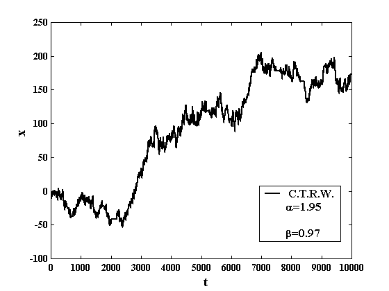
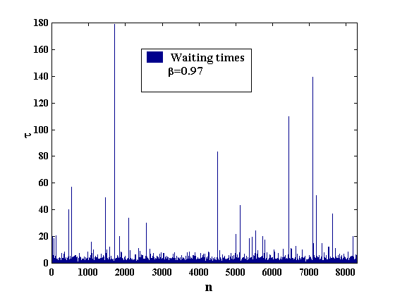
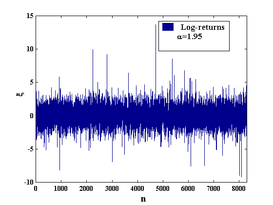
In fig. 1 the log-price x is presented as a function of time t for a simulation of nearly 8300 log-prices. The series of waiting times is plotted in fig. 2 and the log-return series is plotted in fig. 3. In order to check the quality of the distribution, in fig. 4, the "empirical" distribution of waiting times is compared with the theoretical one. The same is done in fig. 5 with the distribution of returns.

In this paper, we have outlined how to simulate and use synthetic markets based on continuous time random walks. In this framework, one has only to find a reasonable approximation of the empirical joint density function j (x ,t ) for each asset, in order to simulate a full market with as many assets as necessary.

There are various possible applications of these simulations. They could be used as well-controlled benchmarks for artificial markets with heterogeneous agents. However, once a large synthetic market is realized, it is possible to use it for other purposes, including portfolio selection, speculative option pricing and scenario generation for value-at-risk analyses

[1] E.W. Montroll and G.H. Weiss, Random walks on lattices II, J. Math. Phys. 6, 167-181, 1965.

[2] E. Scalas, R. Gorenflo and F. Mainardi, Fractional calculus and continuous-time finance, Physica A, 284, 376-384, 2000.

[3] F. Mainardi, M. Raberto, R. Gorenflo and E. Scalas, Fractional calculus and continuous-time finance II: the waiting-time distribution, Physica A, 287, 468-481, 2000.

[4] M. Raberto, E. Scalas and F. Mainardi, Waiting-times and returns in high-frequency financial data: an empirical study, Physica A, 314, 749-755, 2002.

[5] M. Porto and H. E. Roman, Autoregressive processes with exponentially decaying probability distribution functions: Applications to daily variations of a stock market index, Phys. Rev. E. 65, 046149, 2002.

[6] C. Dose, M. Porto, and H. E. Roman, Autoregressive processes with anomalous scaling behavior: Applications to high-frequency variations of a stock market index, Phys. Rev. E, in press.

[7] L. Sabatelli, S. Keating, J. Dudley and P. Richmond, Waiting time distribution in financial markets, Eur. Phys. J. B 27, 273-275, 2002.

[8] J. Masoliver, M. Montero, and G.H. Weiss, Continuous-time random-walk model for financial distributions, Phys. Rev. E 67, 021112/1-9, 2003.

[9] W.H. Press, S.A. Teukolsky, W.T. Vetterling, and B.P. Flannery, Numerical Recipes in C, p.290, Cambridge University Press, Cambridge UK, 2002.

[10] B. Mandelbrot, The variation of certain speculative prices, Journal of Business 36, 394-419, 1963.

[11] R.N. Mantegna and H.E. Stanley, Stochastic process with ultraslow convergence to a Gaussian: the truncated Lévy flight, Phys. Rev. Lett. 73, 2946-2949, 1994.

[12] I. Koponen, Analytic approach to the problem of convergence of truncated Lévy flights towards the Gaussian stochastic process, Phys. Rev. E 52, 1197-1199, 1995.

[13] M.G. Mittag-Leffler, Sur la nouvelle fonction Ea (x), Comptes Rendus Acad. Sci. Paris, 137, 554-558, 1903.

[14] M.G. Mittag-Leffler, Sur la representation analytique d’une branche uniforme d’une fonction monogene. Acta Math. 29, 101-181, 1905.

[15] F. Mainardi and R. Gorenflo, On Mittag-Leffler-type functions in fractional evolution processes, J. Computational and Appl. Mathematics, 118, 283-299, 2000.

[16] A. Erdélyi, W. Magnus, F. Oberhettinger, and F.G. Tricomi, Higher Transcendental Functions, vol. III, Ch. 18, Krieger, Malabar FL, USA, 1981.

Fig. 1: Simulated log-price as a function of time. Both quantities are plotted in arbitrary units. This simulation includes nearly 8300 log-prices. It takes a few seconds to run on an old Pentium II processor at 349 MHz.

Fig 2: Waiting times as a function of the simulation index. The series has been produced by means of the rejection procedure, by comparing [0-1]-uniformly distributed deviates to a probability density of the Mittag-Leffler form with b = 0.97.

Fig. 3: Log-returns as a function of the simulation index. The series has been produced by means of the rejection procedure, by comparing [0-1]-uniformly distributed deviates with a Lévy probability density of index a = 1.95.

Fig. 4: Waiting times: frequency histogram of simulated data compared with theoretical values. This plot is a self-consistency check for the simulation procedure.

Fig 5: Log-returns: histogram of simulated data compared with theoretical values. This plot is a self-consistency check for the simulation procedure.